It’s been awhile that we are waiting for a sensible improvements in Microsoft self-service BI. The good news is that finally there will be some cool new features added to the next version of Excel which is Excel 2016. By some, I mean, well, there not a lot new BI features, but, some. Something is better than nothing, not too bad though!
Integrating BI features with Excel:
Power View and Power Map:
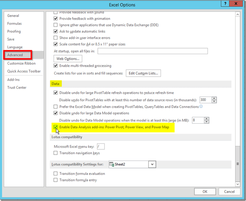
As you know, Power Pivot was integrated as a built-it feature to Excel 2013. Now I’m really happy that the same thing happened to Power View and Power Map. So you don’t need to install them separately. You can now turn these features on from:
File–> Options–> Advanced-> (scroll down the page) Data-> Enable Data Analysis Add-ins: Power Pivot, Power View, and Power Map
OR you can still turn them on from “COM Add-ins”:
File->Options->Add-Ins-> Manage “Com Add-ins”-> Go
Now you can see “Power Map” and “Power View” on the “Insert” tab as well as the “Power Pivot” which has a separate tab:
Power Query:
To me, it’s a very good news that “Power Query” is integrated with Excel. Actually it’s there by default and you don’t even need to turn it on.
You can find it under the “Data” tab on “Get & Transform”:
As you can see I already loaded FactInternetSales query from AdventureWorksDW2012.
When you have a feature as a default feature in Excel you expect to be able to use VBA codes and Power Query is not exception. To see how it works follow the steps below:
- First of all we need enable Developer tab in Excel 2016
- Go to File-> Options-> Customise Ribbon-> tick “Developer”-> OK
- Now you can see the “Developer” tab on the ribbon
- Click “Record Macro”
- Enter a name for the macro then click OK
- Go to Data tab-> Get & Transform-> New Query-> From SQL Server Database
- Enter server and database then click OK
- Select a table then click “Edit”. (Obviously you can directly click on “Load”)
- Follow the steps below to edit the query
- Remove the 5 first key columns by selecting them, right click and “Remove Columns”
- Filter “EndDate” column to show the records with valid end date
- Remove the last 7 columns as well
- Rename the 3 first columns to make them more user friendly
- Click “Close & Load”
- Go back to the “Developer” tab and click “Stop Recording”
- Now click on “Macros” from “Developer” tab
- Click “Edit”
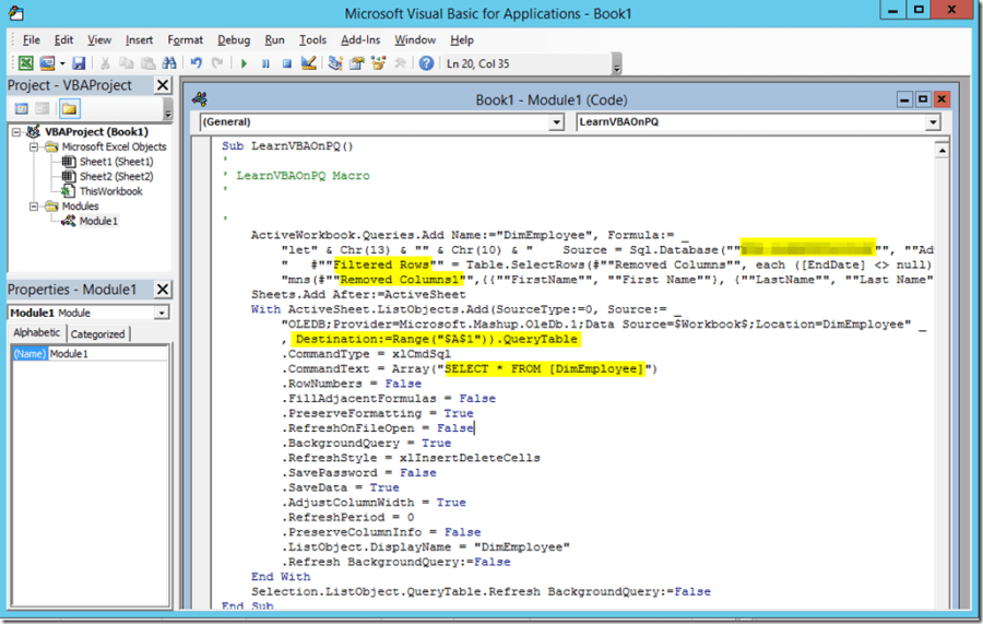
- Here you go, you should be able to see the VBA codes generated over Power Query
You can learn a lot from the recorded codes. If you have a look at the codes you’ll find lots of really interesting codes. You can see all the steps we took when we edited the query like renaming columns and removing columns etc.. You can also see the SQL query which is used to retrieve the data out of the SQL Server database.
But, generally speaking of Power Query in comparison with the latest version of Power Query available for Excel 2013 there is no new features added to it.
Power View Over OLAP (Analysis Services Multi-dimensional):
Another cool feature that’s been added to Excel 2016 is the ability to create “Power View” report on top of OLAP cubes. In the previous version you get the error message below:
“Sorry, Power View in Excel can’t connect to this data source. It may be a multidimensional data source, which Power View doesn’t support yet. Try connecting to a different data source.”
But, in the new version you can create flashy reports on Power View very easily. Just connect to an OLAP data server and import data into a Power View report.
In the sample below we create a report in Power View on top of Adventure Works OLAP cube:
Internet Sales by Full Calendar Date:
Power Pivot:
First of all I really liked the changes on colours and relationship connectors on diagram view.
Now you can rename tables and columns easier by selecting the item and pressing F2 which isn’t enable in Power Pivot 2013. In Power Pivot 2013 you should double click on the object to rename it. If you’re a keyboard guy or girl like me you’ll be happy to have F2 enabled for renaming objects.
You can also rename a table or a column that you added into a Pivot Table from the Model without loosing them from the Pivot Table. As you can see on the screenshot below I renamed DimDate table to Date and I can see the changes straight on the Pivot Table.
When you’re speaking of Power Pivot, there is no way to resist talking about DAX. There are lost of new DAX functions added to Power Pivot 2016. All of these functions are ready to use in Power BI Desktop as well.
You can find new DAX functions here.
That was a brief summary of what are new BI related functionalities in Excel 2016.
Hope you enjoyed it.


Nice post. I was checking continuously this blog and I am impressed!
Very helpful information particularly the last part 🙂 I care
for such info a lot. I was seeking this particular info for a
long time. Thank you and best of luck.